目的:解析iPhone导出的Apple Health 数据文件,分析过往几年的运动轨迹。XML包可以用来处理XML数据:
- 如果把XML看作传统的关系数据库,那么XPath就是SQL。R语言中的XML包可用来解析处理XML或是HTML数据。
- 如果页面中的数据是一个规整的表格,用readHTMLTable函数即可。
- 如果页面中是一些非结构化的数据,就要用到XML包中的其它函数了。其中最重要两个函数是xmlTreeParse()和getNodeSet(),前者负责抓取页面数据并形成树状结构,后者对抓取的数据根据XPath语法来选取特定的节点集合。
数据处理
1 | library(XML) |
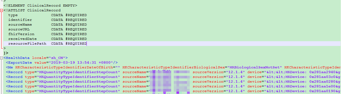
1 | #读取xml文件 |
步数、里程、爬梯数据整理如下:1
2
3
4
5
6
7
8
9
10
11
12
13
14
15
16
17
18
19#步数
StepCount <- healthData[healthData[,1]=="HKQuantityTypeIdentifierStepCount",]
#行走里程
Distance <- healthData[healthData[,1]=="HKQuantityTypeIdentifierDistanceWalkingRunning",]
#楼梯层数
Climbed <- healthData[healthData[,1]=="HKQuantityTypeIdentifierFlightsClimbed",]
#取消科学计数法
options(scipen=200)
#汇总2018年数据(grepl是正则表达式中使用的)
##计算2018年总步数
step_2018 <- sum(StepCount[grepl('^2018',StepCount$date),3])
##计算2018年总里程
dist_2018 <- sum(Distance[grepl('^2018',Distance$date),3])
##计算2018年总楼层
clim_2018 <- sum(Climbed[grepl('^2018',Climbed$date),3])
##计算2018年的天数
day_2018 <- length(unique(StepCount[grepl('^2018',StepCount$date),5]))
在Rmarkdown中,统计18年的总里程数、步数等信息:
2018年已过去r paste(round(day_2018/365*100,0),"%",sep="")(r day_2018天),
累计步行r round(step_2018/10000,2)万步,日平均r round(step_2018/day_2018,0)步;
合计里程r round(dist_2018,2)公里,相当于r round(dist_2018/42.195,2)次全程马拉松;
累计爬楼梯r clim_2018层,约等于r round(clim_2018/100,0)座京基100的楼层数。
按照日期进行统计
1 | #按日期统计 |
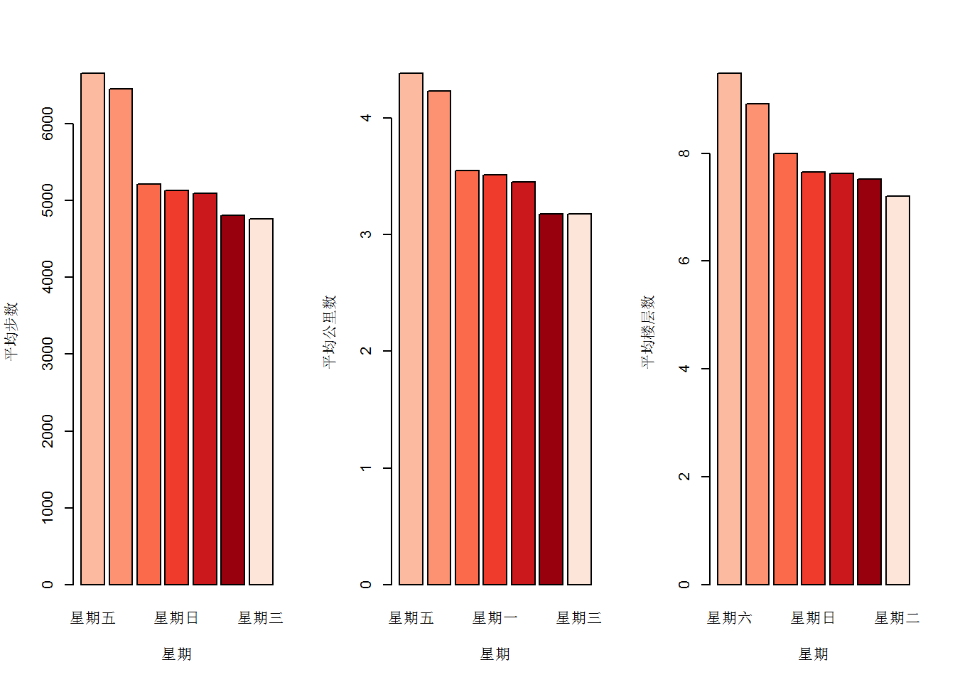
按照星期进行统计
1 | #按日期统计 |
按照月份进行统计
均值、中位数的分月走势1
2
3
4
5
6
7
8
9
10
11
12
13
14
15
16
17
18
19
20
21
22
23
24
25
26
27
28
29
30
31
32
33
34
35
36
37
38
39
40
41#按月度统计
value <- as.numeric(S_date_result)
temp_s <- as.data.frame(value)
temp_s[2] <- format(date_result,"%Y-%m-01")
value <- as.numeric(D_date_result)
temp_d <- as.data.frame(value)
temp_d[2] <- format(date_result_D,"%Y-%m-01")
value <- as.numeric(C_date_result)
temp_c <- as.data.frame(value)
temp_c[2] <- format(date_result_C,"%Y-%m-01")
StepCount_ym <- split(temp_s,temp_s[2],drop=TRUE)
Distance_ym <- split(temp_d,temp_d[2],drop=TRUE)
Climbed_ym <- split(temp_c,temp_c[2],drop=TRUE)
S_ym_result<-lapply(StepCount_ym,FUN=function(x) mean(x$value))
D_ym_result<-lapply(Distance_ym,FUN=function(x) mean(x$value))
C_ym_result<-lapply(Climbed_ym,FUN=function(x) mean(x$value))
SM_ym_result<-lapply(StepCount_ym,FUN=function(x) median(x$value))
DM_ym_result<-lapply(Distance_ym,FUN=function(x) median(x$value))
CM_ym_result<-lapply(Climbed_ym,FUN=function(x) median(x$value))
#分别绘制出“步数、公里数、楼层数”的折线图
par(mfrow=c(1,2))
plot(as.Date(names(S_ym_result)),as.numeric(S_ym_result),type="l",xlab = "月度",ylab = "平均步数",col="#475F77")
plot(as.Date(names(D_ym_result)),as.numeric(D_ym_result),type="l",xlab = "月度",col="#D74B4B",ylim=c(0,15),ylab = "平均公里数 / 楼层数")
lines(as.Date(names(C_ym_result)),as.numeric(C_ym_result),type="l",xlab = "月度",col="#2192BC")
legend("topright",lty=1,bty="n", #去掉框
col=c("red","blue"),
legend=c("平均公里数","平均楼层数"),
cex =0.7) #字体大小
par(mfrow=c(1,2))
plot(as.Date(names(SM_ym_result)),as.numeric(SM_ym_result),type="l",xlab = "月度",ylab = "步数中位数",col="#475F77")
plot(as.Date(names(DM_ym_result)),as.numeric(DM_ym_result),type="l",xlab = "月度",col="#D74B4B",ylim=c(0,15),ylab = "公里数 / 楼层数中位数")
lines(as.Date(names(CM_ym_result)),as.numeric(CM_ym_result),type="l",xlab = "月度",col="#2192BC")
legend("topright",lty=1,bty="n", #去掉框
col=c("red","blue"),
legend=c("公里数中位数","楼层数中位数"),
cex =0.7) #字体大小
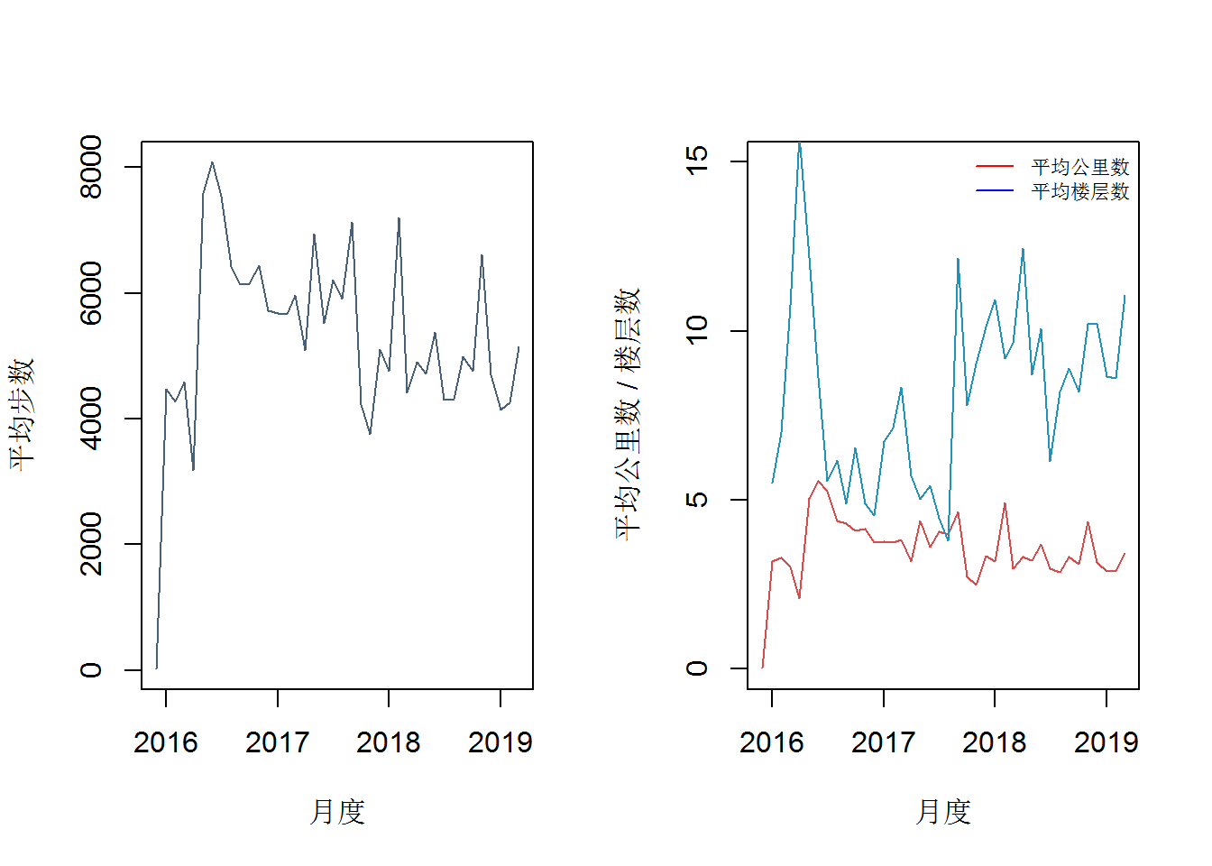
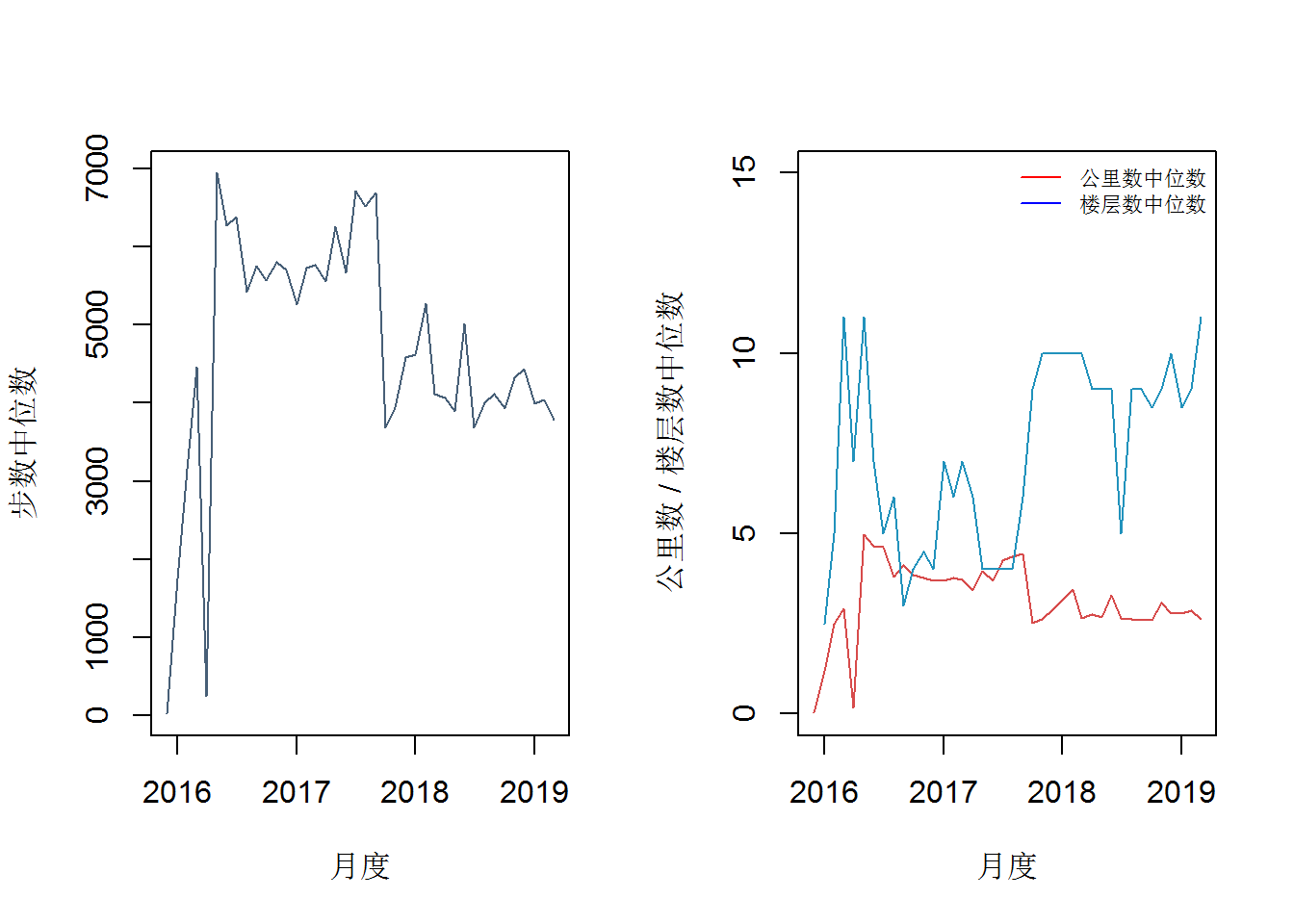
中位数:2018年各月每日步数的中位数基本维持在4000-5000步之间,公里数在3公里左右,楼层数在10层左右;2017年6000步左右,公里数4公里左右,楼层数6层左右
均值:2018年各月每日步数的均值基本维持在6000步之间,公里数在3-公里之间,楼层数也在10层左右
说明:受偏大的异常值影响,均值大于中位数;17年住的地方离地铁站更远一些但是楼层低,18年住的地方距离地铁站近了很多,楼层更高了
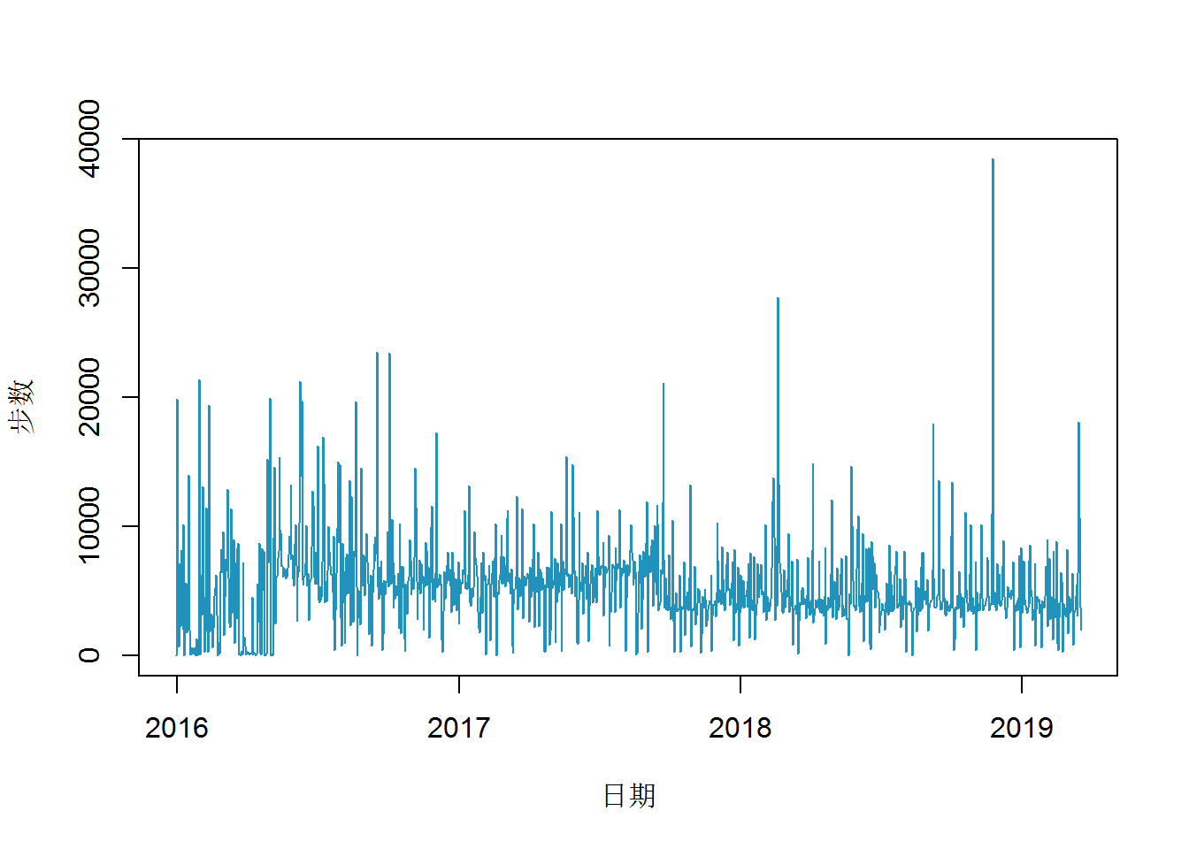
步数图表中加入重要事项标注
标注之前,重新做一个交互式的图,用我们的可视化神器——plotly:1
2
3
4
5
6
7
8
9
10
11
12
13
14
15
16
17
18
19
20
21
22
23p1 <- plot_ly(x=~date_result,y=~as.numeric(S_date_result)) %>%
add_lines(col="#2192BC") %>%
layout(
font = list( family = "Times New Roman",
size = 12,
color = "#444"),
title = '2016-2019年步数记录',
xaxis = list(title='日期'),
yaxis = list(title='步数'),
titlefont = list( family = windowsFont("微软雅黑"),size = 18,
color = '#444'),
autosize = TRUE, # 设置图形大小
width = 700, # 设置图形宽度
height = 400, # 设置图形高度
margin = list(l = 80, r = 80, t = 100, b = 80, pad = 0, autoexpand = TRUE), # 设置图形边界距离
paper_bgcolor = "#fff", # 图表区的背景颜色
plot_bgcolor = "#fff", # x、y轴之间的绘图区的背景颜色
separators = ".,", # 设置小数点和千位数间隔符
showlegend = FALSE, # 是否显示图例
dragmode = "zoom",#"zoom" "pan" "select" "lasso" "orbit" "turntable"
hovermode = "closest" # : "x" | "y" | "closest" | FALSE
)
p1
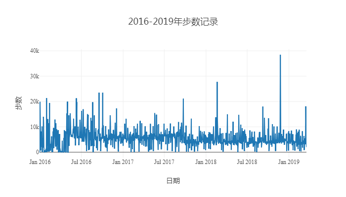
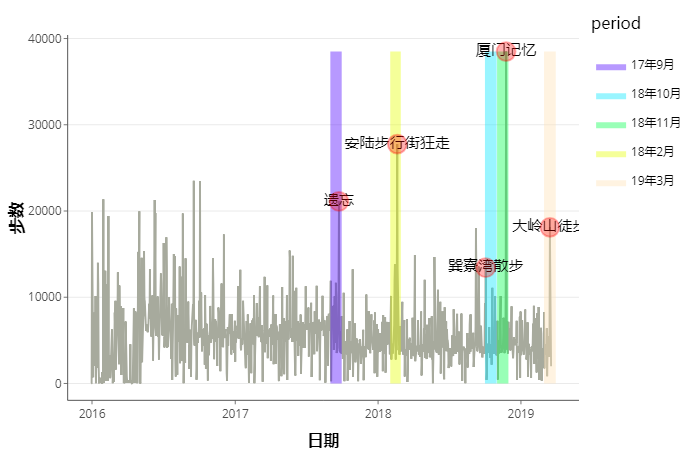
拖拉一下,找到步数大于2万步的日期,回忆下,加上标签:
1 | theme_yj <- |
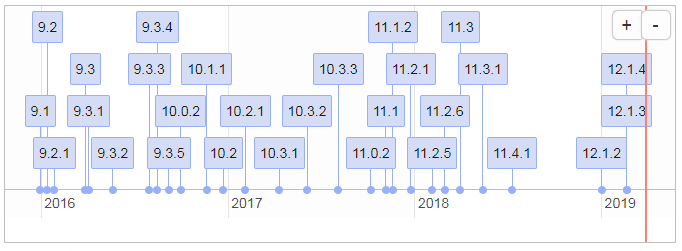
特别的解析
观察数据之后,竟然有个让我惊喜的字段(系统型号),作为一个一直默认自动更新系统的人,每次都是在提示有新版本之后积极的点击刷新。如果不是今年2月发生一件略坑的事件,我大概还是那个积极更换系统的一员。
起因是更新到最新的系统之后,手机没有信号了,作为一个用惯了4G即将迎接5G、一个包里至多也就几十块现金的手机重度依赖者,那个时候是崩溃的。经历了无数次重启、刷机的过程后,依然没有信号……(最后的解决办法,哈哈,请见最后的彩蛋)
1 | select <- dplyr::select |
最长命的系统型号:11.4.1。
| 排序 | 系统型号 | 天数 |
|---|---|---|
| 1 | 11.4.1 | 176 |
| 2 | 9.3.2 | 71 |
| 3 | 10.2.1 | 68 |
| 4 | 10.3.3 | 65 |
| 5 | 10.3.2 | 61 |
最后的彩蛋
- 手机的解决办法:去营业厅换了一个手机卡,所有问题迎刃而解
- timevis包的博文介绍链接
- https://www.cnblogs.com/Hyacinth-Yuan/p/8343425.html